Euler Examples

Search

Rounding Errors

Rounding Errors

by R. Grothmann

This file demonstrates rounding errors. Every computer with a floating point arithmetic makes errors due to rounding. Euler can get rid of some of these errors with the exact scalar product and the interval arithmetic.

First of all, we investigate the basic rounding error.

>a=1/3-0.33333333333333

0

1/3 is not exactly representable in the computer. However, if we multiply it by 3, we get 1 exactly. This is due to the rounding.

>(1/3)*3-1

0

Here is the internal representation of 1/3. In the dual system 1/3 is an infinite series, which is truncated in the computer.

>printhex(1/3)

5.5555555555554*16^-1

(1/3)*3 correctly rounds to 1. This does no longer work for 1/49.

>longestformat; 1/49*49-1, longformat;

-1.110223024625157e-016

By the way, there are not many numbers between 1 and 100 such that 1/n*n does not round to 1.

>n=1:100; nonzeros(1/n*n-1<>0)

[49,  98]

If we use intervals for our computation, we get only an inclusion. This is so, since the division and the multiplication of intervals takes care of rounding errors.

>~1,1~/~3,3~*~3,3~

~0.99999999999999956,1.0000000000000002~

Now we want to demonstrate the propagation of rounding errors.

We iterate sqrt starting from 2 twenty times. The sqrt function is a good function in terms of error propagation. The input error is divided by 2 in each iteration. Thus all values are correct. The left column contains the values generated by iterating sqrt. The right column shows the correct values.

>longestformat; p=iterate("sqrt(x)",2,n=20); p_2^(2^-(1:20))

Real 2 x 21 matrix

                      2     ...
      1.414213562373095     ...

However, going back with x^2 to 2 is not a good function. The error is multiplied by 2 this time. This accumulates to a surprising error.

>longformat; iterate("x^2",p[20],n=20)_2^(2^(-19:1:0))

Real 2 x 21 matrix

      1.00000132207       1.00000264415     ...
      1.00000132207       1.00000264415     ...

This is even more obvious with interval arithmetic.

>p=iterate("sqrt(x)",~2~,20); p=iterate("x^2",p[20],20); p[20]

~1.999999999,2.000000001~

Another example for a rounding error is the subtraction of two large numbers.

>x=10864; y=18817; 9*x^4-y^4+2*y^2,

2

The correct result is 1. We can obtain it in the following way.

>x=10864; y=18817; (3*x^2-y^2)*(3*x^2+y^2)+2*y^2,

1

Of course, Maxima with its infinite arithmetic gets the result exactly.

>:: 9*x^4-y^4+2*y^2 | x=10864 | y=18817

                                  1

By transforming the problem into a linear system, we can get very good results and even inclusions using the exact arithmetic of Euler.

The linear system is v[1]=x, v[2]=x*v[1], ..., v[5]=y, v[6]=y*v[5], ..., v[9]=9*v[4]-v[8]+2*v[2]

>x=10864; y=18817;
>A=id(9);
>A[2,1]=-x; A[3,2]=-x; A[4,3]=-x;
>A[6,5]=-y; A[7,6]=-y; A[8,7]=-y;
>A[9,4]=-9; A[9,8]=1; A[9,6]=-2;
>b=[x, 0, 0, 0, y, 0, 0, 0, 0]';
>v=A\b; v[9],

0

The first solution is wrong.

However, we can improve it with a residual iteration. For this, we compute the error eps=b-A\v and solve the A\e=b, adding this correction to v. However, we need compute eps with higher accuracy. The residuum function does this using Euler's exact scalar product.

>w=v-A\residuum(A,v,b); w[9],

1

This is correct.

The function xlusolve does the same.

>v=xlusolve(A,b); v[9]

1

Using ilgs, which uses a similar trick, we get a bound for the solution.

>v=ilgs(A,b); v[9]

~0.99999999999999978,1.0000000000000002~

We now try the following recursion: I[n+1]=1/(n+1)-5*I[n]. It is true that I[n]=integrate(x^n/(x+5),x,0,1), esp. I[0]=log(1.2). However, we get a large error, since we have to multiply by 5 in each step, which also multiplies the error.

We compute the recursion with the sequence function. Note that the first element of sequence starts with index 1. Thus x[n]=I[n-1].

>sequence("1/(n-1)-5*x[n-1]",log(1.2),21)

[0.182321556794,  0.0883922160302,  0.0580389198489,  0.043138734089,
0.034306329555,  0.0284683522252,  0.0243249055404,  0.021232615155,
0.0188369242248,  0.0169264899873,  0.0153675500637,  0.0140713405907,
0.01297663038,  0.012039925023,  0.0112289463138,  0.0105219350978,
0.00989032451098,  0.00937190685686,  0.00869602127127,
0.00915147259102,  0.00424263704492]

The last number is completely wrong.

>romberg("x^20/(x+5)",0,1)

0.00799752302825

This is even more obvious, if we start with intervals.

>v=sequence("1/(n-1)-5*x[n-1]",log(~1.2~),21); v[-1]

~-0.022,0.03~

However, if we compute the recursion backwards, we get I[0] exactely, even if we start very far off of I[20].

The reason is, that the error divides by 5 in each step.

>v=sequence("0.2*(1/(20-n)-x[n-1])",0,19); v[-1]

0.182321556794

>log(1.2)

0.182321556794

Indeed, we get an inclusion for the value, if we start with any interval containing I[20].

>v=sequence("0.2*(1/(20-n)-x[n-1])",~0,1~,19); v[-1]

~0.18232155679395,0.18232155679422~

Euler has a function for the Chebyshev polynomials. "cheb" computes the polynomial the fastest way. We test it for degree 60 at 0.9.

>cheb(0.9,60)

-0.350468376614

There is also a recursive routine for the Chebyshev polynomials. The recursive version is very exact. This is surprising in view of the example above.

>chebrek(0.9,60)

-0.350468376614

However, if we compute the polynomial and evaluate it at 0.9 with polyval, the result is completely wrong.

>p=chebpoly(60); ...
 evalpoly(0.9,p)

-14447.2139393

This is not due to the coefficients, as we see with interval aritmetic. The function ipolyval computes inclusions for polynomials using residuum arithmetic.

>ievalpoly(0.9,p)

~-0.3504683772,-0.350468376~

xpolyval is faster, but less reliable.

>xevalpoly(0.9,p)

-0.350468376613

The small remaining difference to the correct value is due to the coefficients.

>cos(60*acos(0.9))

-0.350468376614

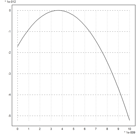
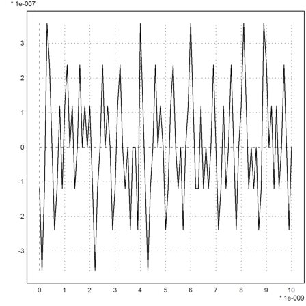
Another example is the following polynomial due to Rump.

>p=[-945804881,1753426039,-1083557822,223200658];

We evaluate it in the following interval.

>t=linspace(1.61801916,1.61801917,100);

The values are clearly wrong.

>plot2d(t-1.61801916,evalpoly(t,p)):

The correct values are easily obtained with a little residual iteration.

>plot2d(t-1.61801916,xevalpoly(t,p,eps=1e-17)):

Examples